This post is the third in a series of three blog posts that cover the basics of running R in Docker. The three parts are:

• Part 1: Running R in Docker containers interactively and as server processes
• Part 2: Extending Rocker images to install packages
• Part 3: Knitting RMarkdown in containers for reproducible research

In this final post, we look at a common scenario: using R in Docker to encapsulate a research objective or task in an RMarkdown document and knit that document in a container with specific versions of R and supporting packages.

Example Scenario

I initially developed this scenario as part of my tutorial on using R and Docker together at the 2018 useR! Conference (slides, video). Since the conference was in Australia, I chose the 2016 Australian Federal election as the illustrative "research topic". The goal here is to provide an example that shows how to use Docker to reproduce research, not to perform a comprehensive analysis of the election. With that in mind, the analysis seeks to visualize the relationship between the 2016 unemployment rate in each Commonwealth Electoral District in Australia and the share of the final vote won by the incumbent Liberal coalition in each district.

To simplify the scenario further, we handle the download and preparation of the data from the Australia Election Commission in a separate step. The analysis notebook consumes the prepared data from a dataset on data.world's collaboration platform (free signup required to see the dataset details on the platform, but you can download the files as csv (election results, census data) without logging in.) The code for the data download and preparation is available in GitHub.

In this example, the analysis consists of a single RMarkdown notebook and our goal is to knit it into html for publication online.

Brief Detour: Docker Volumes and Persisting Container State

Typically, we want to save the results of our analysis for publication or further use. However, once a Docker container is removed (including automatically with the --rm option to docker run), any changes to the container file system are discarded. This is in keeping with the Docker philosophy that containers should be stateless--that is, that any file whose state should live beyond the lifetime of the container should be stored outside the container. Docker volumes provide a mechanism for managing this kind of container-independent storage.

In this example, we will use bind mount volumes, as they are best suited to easy recovery of files created in a container. When setting up a bind mount, we specify a location on the host as the source of the mount. Docker also provides volume mount volumes, whose locations are managed by Docker and are somewhat trickier to access. You can read more about volumes on the Docker website.

We use bind-mount volumes by passing a --mount command-line option to docker run with a type of "bind". For instance, to mount the directory /analysis-output in a base R container and "point" that directory to directory /Users/scott/Documents/analysis-output on my host (I'm on a Mac), I could do the following:

$: mkdir -p /Users/scott/Documents/analysis-output
$: docker run -it --rm --mount "type=bind,source=/Users/scott/Documents/analysis-output,target=/analysis-output" rocker/r-ver:3.5.1

R version 3.5.1 (2018-07-02) -- "Feather Spray"
Copyright (C) 2018 The R Foundation for Statistical Computing
Platform: x86_64-pc-linux-gnu (64-bit)

R is free software and comes with ABSOLUTELY NO WARRANTY.
You are welcome to redistribute it under certain conditions.
Type 'license()' or 'licence()' for distribution details.

R is a collaborative project with many contributors.
Type 'contributors()' for more information and
'citation()' on how to cite R or R packages in publications.

Type 'demo()' for some demos, 'help()' for on-line help, or
'help.start()' for an HTML browser interface to help.
Type 'q()' to quit R.

> dir.exists('/analysis-output')
[1] TRUE
> write.csv(data.frame(a=1:5), '/analysis-output/data.csv', row.names=FALSE)
> quit()
$: 

Then, back on my host, I could do the following to verify that the file remains after the container is gone:

$: cat /Users/scott/Documents/analysis-output/data.csv
"a"
1
2
3
4
5

Now that we know how to bind-mount a volume, we're ready to build our image and run our analysis so that the output is saved for consumption or publication.

Building the Image

In Part 2 we saw how to create a Dockerfile that defines an extension of a Rocker project image that tailors an R environment to a specific project's needs. We will follow that same approach here, but in addition to installing packages that we need (like we did in Part 2), we will also install the source code for our notebook so it's available when we run the container.

Here is the Dockerfile:

FROM rocker/tidyverse

VOLUME /analysis-output

RUN R -e 'install.packages(c("ggthemes", "scales"))'
RUN mkdir /analysis-source
COPY Notebook.Rmd /analysis-source/

CMD ["R", "-e", "rmarkdown::render('/analysis-source/Notebook.Rmd', output_file='/analysis-output/Notebook.html')"]

Make sure this Dockerfile lives in the same directory as Notebook.Rmd (and any other files referenced in a COPY instruction) and then build with docker build -t [image-name] .. As we saw in Part 2, we can install any R packages we need by running R -e ... during the assembly process.

The key instruction here is CMD. It specifies that the default executable for containers run from this image will be run the one-line R program rmarkdown::render(...). The render() function simply knits the file found at the first argument, and as invoked here, writes output to the specified output_file location. Note that we point output_file to the volume mount point, which is linked to a host directory at container runtime.

If we wanted to take the image a step further, we could push it to an account on DockerHub, so that others who wish to reproduce our results only need to pull the image rather than build it. To push this image, we first tag it to qualify the image name with an account, then use docker push to upload it:

$: docker tag australia-federal-2016 scottcame/australia-federal-2016
$: docker push scottcame/australia-federal-2016
The push refers to repository [docker.io/scottcame/australia-federal-2016]
818c625b7757: Pushed
...
latest: digest: sha256:72bf71a3b5841dc0f06d2d28396cc6d86c09de78574ffc971d8c65b0653f5a7d size: 2417
$: 

Organizing your Code

It is often easiest--especially for very simple notebooks--to place the Dockerfile in the same directory as the notebook and manage the entire codebase in a source control system like GitHub. Just be aware that docker build ... copies the entire build context directory to the image context. If you have lots of other files in the directory that are irrelevant to the notebook, you can leave them out of the Docker build context by listing them (specifically or by pattern) in a .dockerignore file. Maintaining the Dockerfile and notebook source code together helps to keep them in sync and avoids having another step to bring all the artifacts together for the build.

You can see an example of this in the GitHub repository for this example.

Docker and Improved Reproducibility

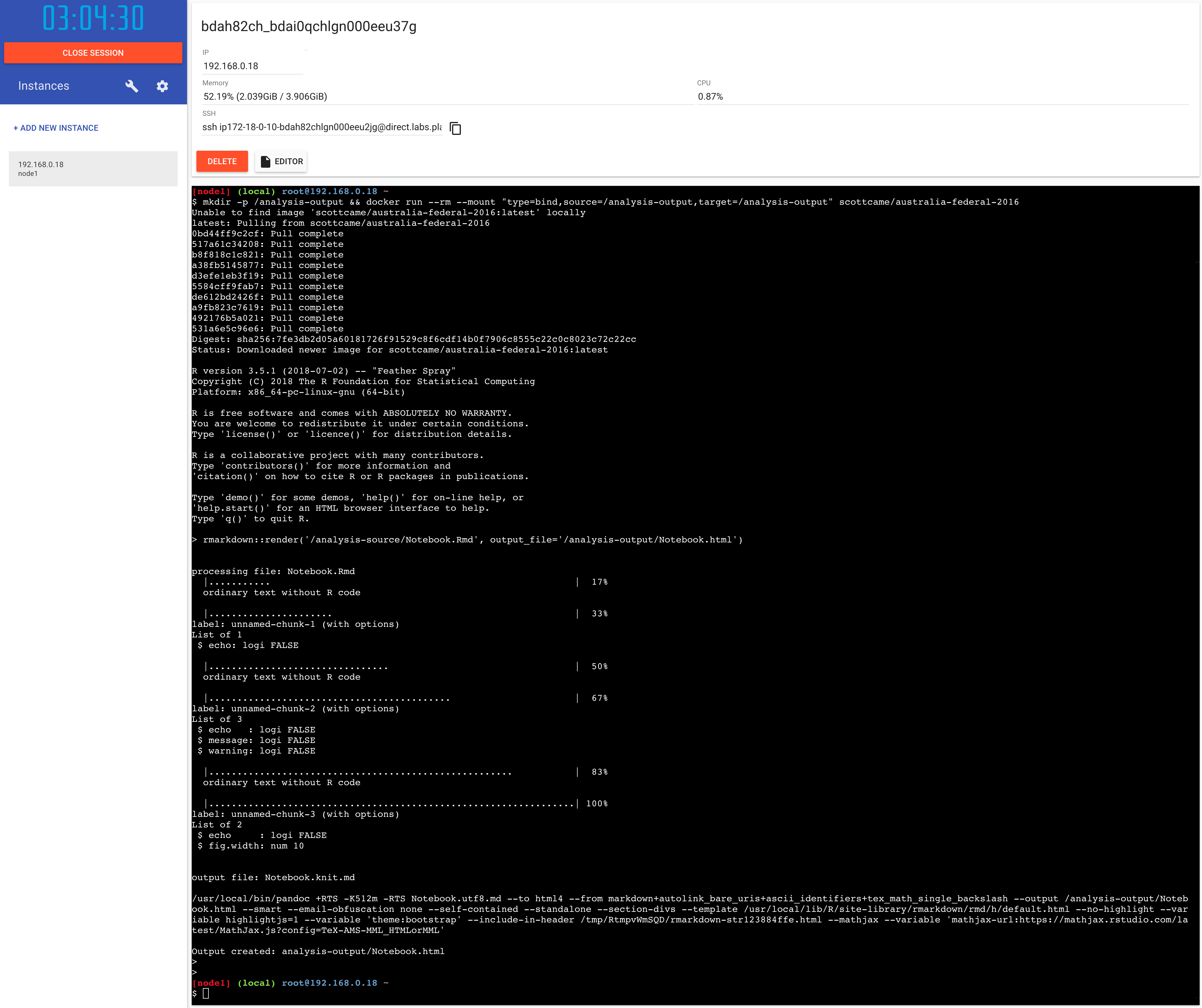
Docker allows us to encapsulate a research pipeline and context in a single artifact--the Dockerfile--that allows others to produce our results without having to follow lengthy (and error-prone) installation instructions. A fellow researcher need only have Docker installed and run a single command. In fact, Play with Docker allows us to reproduce these results without even having Docker installed locally:

We can even run an http server like Apache on Play with Docker to see the output, again making use of bind mounts to make our /analysis-output directory the place from which Apache serves up static web content:

$: docker run -d --rm --mount "type=bind,source=/analysis-output,target=/usr/local/apache2/htdocs/" -p 80:80 httpd:2.4

Or, from your local machine, you can simply curl it:

$: curl -s -O http://ip172-18-0-10-bdah82chlgn000eeu2jg.direct.labs.play-with-docker.com/Notebook.html

Note that Play with Docker makes Docker services available at an Internet address that's the same as the SSH endpoint with the "@" changed to a dot. The SSH endpoint is shown above the shell area for each PWD instance.

I've shown Play with Docker here because it is a really useful resource for experimentation and testing things out. Of course, in a real research scenario, we're more likely to use Docker on a private cloud server or on our own desktop.